![]()
Gecko generalized phylogenetics
Objective
Our goal is to learn how to set up, run, and interpret a phycoeval analysis in order to infer phylogenies with shared and multifurcating divergences.
Background Information
Biogeographers are often interested in understanding how environmental changes affect diversification. When such processes simultaneously affected multiple ancestral species, this can produce patterns of shared divergences. Phycoeval provides a tool for testing such predictions using a fully phylogenetic Bayesian model choice approach [20].
For more detailed background information about the method implemented in phycoeval, please see here.
Software Used in this Activity
For this activity, we will be using phycoeval (part of the ecoevolity package). If you haven’t already done so, please follow the instructions for installing ecoevolity. Either installing ecoevolity directly or using the Docker image will work for this tutorial.
While not required, you may want to install the program Tracer (https://github.com/beast-dev/tracer/releases), a nice tool for visualizing the mixing and convergence behavior of Markov chain Monte Carlo (MCMC) analyses.
Getting the example files for this tutorial
We will use git to download the data and phycoeval configuration file we need
for this tutorial.
To do this open your preferred shell (command-line) environment (e.g., Bash),
and type the following two commands to download a directory (“folder”)
with the data
and move into it:
git clone https://github.com/joaks1/phycoeval-example-data.git
cd phycoeval-example-data
Extra steps for Docker users
If you are using the Docker container to run phycoeval, follow these two extra
steps to be able to analyze the example files you just downloaded.
First, make sure you are NOT inside the Docker container before
proceeding; you want to be at your computer’s command-line console.
After you’ve used cd to navigate into the phycoeval-example-data
directory we created above, execute the following command to enter the
Docker container:
docker run -v "$(pwd)":/portal -it phyletica/ecoevolity-docker bash
Note
Depending on your system and how Docker is configured, you may need to use
sudo to run Docker commands. If you received a “permission denied”
message when you ran the command above, try:
sudo docker run -v "$(pwd)":/portal -it phyletica/ecoevolity-docker bash
Then, once inside the Docker container, type:
cd portal
For the remainder of the tutorial, enter (or copy and paste) any command-line instructions into the command line of the Docker container. However, you can view and edit the input and output files on your computer (outside the container) with your plain text editor of choice.
When you list the contents of the phycoeval-example-data using ls,
you should see the following files:
Cyrtodactylus-tutorial-data.nexThis file contains nexus-formatted RADseq data comprising 50 loci from 7 bent-toed geckos (Cyrtodactylus) from insular populations in the Philippines. For detailed information about how to format nexus files for phycoeval, click here.
phycoeval-config.ymlThis is a YAML-formatted configuration file that will tell phycoeval how to analyze the data.
README.mdYou can ignore this file.
The Data
We will be analyzing 50 RADseq loci from 7 insular populations of bent-toed geckos (Cyrtodactylus) from the Philippines. This is a small subset of the data analyzed in [20]. Phycoeval assumes our characters have two-states (biallelic) and are unlinked.
Biallelic characters
Phycoeval assumes all of your characters have at most two states (biallelic).
If we provide phycoeval with nucleotide data, it will automatically recode the data
as biallelic by considering the first character it finds in each column as
state 0, and if it finds a second state it considers it state 1.
If it finds a third state in a column, it will report an error message and
quit.
For characters (columns) with more than two states, you have two options:
remove these columns from your matrix, or
recode them as biallelic.
Phycoeval will do the latter for you (more on this in a bit).
Linked characters
Phycoeval also assumes all your characters are unlinked. Based on analyses of data simulated with linked characters [20], we recommend that you analyze all of your characters (including the constant ones) and violate the assumption of unlinked characters. In short, phycoeval performs better when you use all of the sites (including the constant ones) compared to reducing the data to only (effectively) unlinked variable characters. The example data sets we’ll be analyzing consist of 50 loci each comprising about 90 linked sites.
Setting up the phycoeval configuration file
Once we have our nexus-formatted data ready, the next step in an phycoeval analysis is setting up the configuration file. Phycoeval requires a YAML-formatted configuration file. YAML is a human-friendly data standard that allows you to provide phycoeval the information it needs in a format that is easy for you to read and edit.
Note
The website http://www.yamllint.com/ is a nice tool for debugging YAML syntax. You can copy and paste your config file there to check if you’re using valid YAML syntax.
For detailed information about all the settings that can be included in an phycoeval config file, click here.
In the phycoeval-example-data directory, there is a YAML-formatted
config file named phycoeval-config.yml, which contains the following
information:
---
data:
    ploidy: 2
    constant_sites_removed: false
    alignment:
        genotypes_are_diploid: true
        markers_are_dominant: false
        population_name_is_prefix: false
        population_name_delimiter: ' '
        path: Cyrtodactylus-tutorial-data.nex
mutation_parameters:
    mutation_rate:
        value: 1.0
        estimate: false
    freq_1:
        value: 0.5
        estimate: false
branch_parameters:
    population_size:
        equal_population_sizes: true
        value: 0.0005
        estimate: true
        prior:
            gamma_distribution:
                shape: 4.0
                mean: 0.0005
tree_model:
    tree_space: generalized
    starting_tree: comb
    tree_prior:
        uniform_root_and_betas:
            parameters:
                root_height:
                    estimate: true
                    prior:
                        exponential_distribution:
                            mean: 0.01
mcmc_settings:
    chain_length: 7500
    sample_frequency: 5
Let’s break this down to go over all the settings specified in this config.
First, the data section.
data
data:
    ploidy: 2
    constant_sites_removed: false
    alignment:
        genotypes_are_diploid: true
        markers_are_dominant: false
        population_name_is_prefix: false
        population_name_delimiter: ' '
        path: Cyrtodactylus-tutorial-data.nex
This section tells phycoeval all about our data, including:
the geckos are diploid (
ploidy: 2),we have not removed constant sites from the alignment,
each cell in the alignment represents the genotype of a diploid individual (
genotypes_are_diploid: true),our nucleotide data are not dominant (i.e., we can distinguish heterozygous genotypes for a site from either of the two homozygous genotypes),
the last part of every sequence label specifies the population/species it belongs to (
population_name_is_prefix: false), andthe data are found in a file named
Cyrtodactylus-tutorial-data.nexin the current directory
mutation_parameters
The mutation_parameters section specifies that we wish to fix the rate of
mutation to 1:
mutation_rate:
    value: 1.0
    estimate: false
This means that time will be measured in expected substitutions per site,
and effective population sizes will be scaled by the mutation rate
( ).
).
We also constrain the equilibrium frequencies of the two possible states for each character to be equal:
freq_1:
    value: 0.5
    estimate: false
If you are analyzing nucleotide data, this is almost certainly what you want to do. Phycoeval assumes biallelic data, and there are many ways to convert 4-state nucleotide data into 2-states. If we don’t constrain the frequencies to be equal, our results might vary depending on how choose to do this conversion.
branch_parameters
The branch_parameters section specifies how we wish to model
the effective population sizes of branches across the tree:
population_size:
    equal_population_sizes: true
    value: 0.0005
    estimate: true
    prior:
        gamma_distribution:
            shape: 4.0
            mean: 0.0005
The equal_population_sizes: true setting specifies that
all the branches share the same effective population size.
We specify a starting value for this parameter (value: 0.0005),
and that we wish to estimate it from the data.
Lastly, we specify a gamma-distributed prior distribution on the population
size with a shape and mean of 4 and 0.0005, respectively.
Because the mutation rate is fixed to 1 (see mutation_parameters above),
the effective population size is scaled by the mutation rate,
so we are putting a prior on
.
tree_model
Next, the tree_model section specifies how we want phycoeval to model trees:
tree_model:
    tree_space: generalized
    starting_tree: comb
    tree_prior:
        uniform_root_and_betas:
            parameters:
                root_height:
                    estimate: true
                    prior:
                        exponential_distribution:
                            mean: 0.01
This tells phycoeval to allow “generalized” trees with shared and multifurcating
divergences (i.e., all possible non-reticulating tree models),
and to begin the MCMC chain with the comb tree (the tree where
all tips diverge from a single internal node).
The only tree_prior implemented in phycoeval is the
uniform_root_and_betas tree prior,
which is
described in more detal here.
Lastly, this section specified how to model the age of the root node
(root_height).
This config specifies that we want to allow the age of the root to vary
(estimate: true),
and we are placing an exponentially distributed prior distribution on
it with a mean of 0.01.
Given that the mutation rate is fixed to 1 (see mutation_parameters section
above), this is in units of expected substitutions per site.
How to calibrate time?
Scaling to absolute time...
Currently in phycoeval there are only two ways to calibrate time to be in units
other than substitutions per site (e.g., years or millions of years).
You can place an informative prior distribution on either the
root age or the mutation rate (or both).
If you do this, it is important to remember that the root_height,
mutation_rate, and population_size are all interrelated.
So, changing the setting for one of them, probably requires adjusting
all three of these settings. Let’s walk through an example to
make this clearer.
Let’s say we have prior data about the mutation rate of our Philippine bent-toed geckos. Based on these prior data, we are very confident the rate of mutation of our RADseq loci is 0.001 substitutions per site per million years. So, we decide to put an informative prior on the rate of mutation per million years:
mutation_rate:
    value: 0.001
    estimate: true
    prior:
        gamma_distribution:
            shape: 100.0
            mean: 0.001
That’s great, but now we need to change our settings for the root age and
population size accordingly.
Time is now in millions of years, rather than expected substitutions
per site like it was above when  .
Above, when , our prior expectation for the age of the root
was 0.01 substitutions per site.
Now, we expect the rate of mutation is 0.001 substitutions per million years,
so our new expectation for the age of the root is
.
Above, when , our prior expectation for the age of the root
was 0.01 substitutions per site.
Now, we expect the rate of mutation is 0.001 substitutions per million years,
so our new expectation for the age of the root is
 million years.
So we should change our prior on the
million years.
So we should change our prior on the root_height to something like:
root_height:
    estimate: true
    prior:
        exponential_distribution:
            mean: 10.0
Also, when ,
our prior expectation for the mutation-scaled effective population size
() was 0.0005.
Now that we expect a rate of mutation of 0.001 substitutions per million
years, we have to adjust our prior on the population size:

So, we should also change our prior on population_size to something like:
population_size:
    equal_population_sizes: true
    value: 0.5
    estimate: true
    prior:
        gamma_distribution:
            shape: 4.0
            mean: 0.5
For more about specifying settings for population size parameter(s), see here.
Running phycoeval
Now that we have our nexus-formatted data file and YAML-formatted config file ready, now we will use phycoeval to infer the phylogeny of our 7 geckos, including potentially shared or multifurcating divergences. First let’s take a look at the help menu of phycoeval:
phycoeval -h
If phycoeval is correctly installed, you should get output that looks something like:
======================================================================
                              Phycoeval
                  Estimating phylogenetic coevality

                               Part of:
                              Ecoevolity
        Version 1.1.0 (dev 041c63a: 2026-01-06T13:06:07-06:00)
======================================================================

Usage: phycoeval [OPTIONS] YAML-CONFIG-FILE

Phycoeval: Estimating phylogenetic coevality

Options:
  --version             show program's version number and exit
  -h, --help            show this help message and exit
  --seed=SEED           Seed for random number generator. Default: Set from clock.
  --ignore-data         Ignore data to sample from the prior distribution.
                        Default: Use data to sample from the posterior distribution
  --nthreads=NTHREADS   Number of threads to use for likelihood calculations.
                        Default: 1 (no multithreading). If you are using the
                        '--ignore-data' option, no likelihood calculations
                        will be performed, and so no multithreading is used.
  --prefix=PREFIX       Optional string to prefix all output files.
  --relax-constant-sites
                        By default, if you specify 'constant_sites_removed =
                        true' and constant sites are found, phycoeval throws
                        an error. With this option, phycoeval will
                        automatically ignore the constant sites and only issue
                        a warning (and correct for constant sites in the
                        likelihood calculation). Please make sure you
                        understand what you are doing when you use this option.
  --relax-missing-sites
                        By default, if a column is found for which there is no
                        data across all populations, phycoeval throws an
                        error. With this option, phycoeval will automatically
                        ignore such sites and only issue a warning.
  --relax-triallelic-sites
                        By default, if a DNA site is found for which there is
                        more than two nucleotide states, phycoeval throws an
                        error. With this option, phycoeval will automatically
                        recode such sites as biallelic and only issue a
                        warning. These sites are recoded by assigning state 0
                        to the first nucleotide found and state 1 to all
                        others. If you do not wish to recode such sites and
                        prefer to ignore them, please remove all sites with
                        more than two nucleotide states from your DNA
                        alignments. NOTE: only alignments of nucleotides are
                        affected by this option, not alignments of standard
                        characters (i.e., 0, 1, 2).
  --dry-run             Do not run analysis; only process and report settings.
In addition to the settings in our YAML config file, this help menu shows us
what options for phycoeval we can specify on the command line.
NOTE: if you did not compile ecoevolity to allow multi-threading, you will not
see the --nthreads option.
Let’s try running an analysis with phycoeval:
phycoeval phycoeval-config.yml
Oops, we got an error:
#######################################################################
###############################  ERROR  ###############################
21 sites from the alignment in:
    'Cyrtodactylus-tutorial-data.nex'
have no data across all populations.
#######################################################################
This error message is telling us that we have 21 sites (columns) in our character matrix for which we have no data for any of our samples (rows). Such sites can be common when we subsample individuals from a larger dataset. Rather than removing these sites ourselves, we can tell phycoeval to ignore them.
Before we do that, let’s talk about another common error you might see with your own data that will look something like (you won’t get this error for the example data):
#######################################################################
###############################  ERROR  ###############################
7 sites from the alignment in:
    'Cyrtodactylus-tutorial-data.nex'
have more than two character states.
#######################################################################
This error message is telling us that we have 7 sites (columns) in our character matrix where there are more than two states represented across our samples. As discussed above, at this point, we have 2 options:
Remove any characters with more than two states.
Recode these sites as biallelic.
The latter phycoeval will do for us if we specify the
--relax-triallelic-sites option in our command.
When we use this option, phycoeval will consider the first state in a column as
0, and any other state found in the column as 1.
OK, let’s try running phycoeval again, but tell it to ignore the 37 sites for which at least one population has no data:
phycoeval --relax-missing-sites phycoeval-config.yml
Now, you should be running! How long the analysis takes to run will depend on your computer, but it took about 2 minutes on my laptop.
Checking the pre-MCMC screen output
While the analysis is running, let’s scroll up in our console and look at the information phycoeval reported before the MCMC chain started sampling. This output goes by very quickly, but it’s very important to read it over to make sure phycoeval is doing what you think it’s doing. At the very top, you will see something like:
======================================================================
                              Phycoeval
                  Estimating phylogenetic coevality

                               Part of:
                              Ecoevolity
        Version 1.1.0 (dev e4f5e39: 2026-01-07T21:52:17-06:00)
======================================================================

Seed: 2036173920
Using data in order to sample from the posterior distribution...
Config path: phycoeval-config.yml
This gives us detailed information about the version of ecoevolity we are using
(right down to the specific commit SHA).
It also tells us what number was used to seed the random number generator; we
would need to provide phycoeval this seed number using the --seed
command-line option in order to reproduce our results.
The output is also telling us that phycoeval is using the data to sample from the
posterior, as opposed to ignoring the data to sample from the prior.
We can do the latter by specifying the --ignore-data command-line option.
Next, phycoeval reports a fully specified YAML-formatted configuration file to the screen. It’s always good to look this over to make sure phycoeval is configured as you expect.
Next, you will see a summary of the data:
----------------------------------------------------------------------
Summary of data from 'Cyrtodactylus-tutorial-data.nex':
    Genotypes: diploid
    Markers are dominant? false
    Number of populations: 7
    Number of sites: 4554
    Number of variable sites: 104
    Number of patterns: 34
    Patterns folded? true
    Population label (max # of alleles sampled):
        philippinicusSibuyan (2)
        philippinicusPanay (2)
        philippinicusNegros (2)
        philippinicusMindoroELR (2)
        philippinicusMindoroRMB (2)
        philippinicusTablas (2)
        philippinicusLuzonCamarinesNorte (2)
----------------------------------------------------------------------
It is very important to look over this summary to make sure phycoeval “sees” your data the way you expect it should. Make sure the number of sites, the number of populations, and the number of alleles per population match your expectations! It is very easy to have typos in your population labels that result in extra tip populations/species you didn’t intend.
Next, phycoeval reports how many threads it is using and where it is logging information about sampled trees, parameter values, and MCMC operator statistics:
Number of threads: 1
Tree log path: phycoeval-config-trees-run-1.nex
State log path: phycoeval-config-state-run-1.log
Operator log path: phycoeval-config-operator-run-1.log
Next, phycoeval reports a summary of the state of the MCMC chain to the screen for
every 10th sample it’s logging to the output files.
After the chain finishes, phycoeval also reports statistics associated with all
of the MCMC operators; this information is also logged to the file specified
above as the Operator log path.
The Output Files
After the analysis finishes, type ls at the command line:
ls
You should see three log files that were created by phycoeval:
phycoeval-config-trees-run-1.nexphycoeval-config-state-run-1.logphycoeval-config-operator-run-1.log
If you open the operator log with a plain text editor, you’ll see this file
contains information about the MCMC operators.
If you have convergence or mixing issues, this information can be useful for
troubleshooting.
If you open the state file, you’ll see it contains the log likelihood,
prior, and parameter values associated with each MCMC sample.
Running additional chains
Before we start summarizing the results, let’s run a second chain so we can assess convergence and boost our posterior sample size. If you have multiple cores on your computer and you’ve compiled ecoevolity to allow multi-threading, let’s tell phycoeval to use two threads for the second MCMC analysis:
phycoeval --nthreads 2 --relax-missing-sites phycoeval-config.yml
Now’s a good time to go grab a coffee, while you wait for the second chain to finish running. With 2 threads, it takes about 70 seconds on my laptop.
After the chain finishes, if you use ls you should see the
following run-2 log files:
phycoeval-config-trees-run-2.nexphycoeval-config-state-run-2.logphycoeval-config-operator-run-2.log
Two MCMC chains is enough to proceed with this tutorial, but for “real” analyses, I recommend doing more. It increases your sample size from the posterior distribution and allows you to better assess convergence.
I ran 2 additional chains (4 total) on my computer, however, you can proceed with the steps below with only 2.
Summarizing the Results
Assessing convergence and mixing
Before summarizing our posterior sample of trees and other parameter values, we will use the sumphycoeval command-line tool to assess whether our MCMC chains converged and mixed well, and if so, how many samples should we ignore from the beginning of each chain before they converged (i.e., “burn-in” samples). If you enter the following command:
sumphycoeval -h
you should see the help menu of sumphycoeval printed to your terminal screen,
showing all the command-line options available for this tool.
The first option we will use to help assess convergence and mixing is the
-c option.
This tells sumphycoeval that we want it to report statistics for assessing
convergence and mixing for different levels of burn-in (i.e., ignoring
different numbers of samples from the beginning of each MCMC chain).
The number we provide after -c tells sumphycoeval the interval (in
numbers of samples) we want between the different burn-in values.
Enter the following command to have sumphycoeval create a tab-delimited table
of convergence statistics where each row is ignoring a larger number of samples
from the beginning of each chain, incrementing by 100 samples:
sumphycoeval -c 100 phycoeval-config-trees-run-?.nex > convergence-stats.tsv
After this command finishes, you can open the convergence-stats.tsv with
a text editor or any spreadsheet program (e.g., Excel) to view the table of
convergence statistics.
It should look something like:
burnin |
sample_size |
asdsf |
psrf_tree_length |
psrf_root_height |
psrf_root_pop_size |
ess_tree_length |
ess_root_height |
ess_root_pop_size |
|---|---|---|---|---|---|---|---|---|
1 |
6000 |
0.0100968 |
1.00437 |
1.00578 |
1.00061 |
561.078 |
510.362 |
1164.36 |
101 |
5600 |
0.00919807 |
1.0005 |
1.00109 |
1.00072 |
1559.35 |
1355.05 |
943.532 |
201 |
5200 |
0.00934073 |
0.999967 |
1.00028 |
1.00026 |
1667.86 |
1391.76 |
1091.25 |
301 |
4800 |
0.00861836 |
1.00019 |
1.00071 |
1.00027 |
1684.37 |
1538.8 |
985.953 |
401 |
4400 |
0.0088828 |
1.0004 |
1.00118 |
1.00082 |
1523.88 |
1358.56 |
865.223 |
501 |
4000 |
0.0109959 |
1.00231 |
1.00317 |
1.00226 |
1207.2 |
1067.46 |
897.208 |
601 |
3600 |
0.0105226 |
1.00464 |
1.00558 |
1.00242 |
1439.17 |
1171.66 |
816.354 |
701 |
3200 |
0.0113964 |
1.00584 |
1.00728 |
1.00503 |
955.667 |
796.888 |
611.316 |
801 |
2800 |
0.0124932 |
1.00761 |
1.00924 |
1.00812 |
766.245 |
708.327 |
612.286 |
901 |
2400 |
0.0155171 |
1.00628 |
1.00822 |
1.00753 |
870.181 |
698.155 |
634.201 |
1001 |
2000 |
0.0173652 |
1.0056 |
1.00874 |
1.0083 |
553.268 |
505.993 |
450.036 |
1101 |
1600 |
0.0185453 |
1.00784 |
1.01091 |
1.00841 |
540.942 |
429.984 |
424.32 |
1201 |
1200 |
0.0176997 |
1.00433 |
1.00549 |
1.01137 |
442.59 |
406.633 |
288.246 |
1301 |
800 |
0.0218634 |
1.01391 |
1.01288 |
1.01959 |
262.872 |
258.65 |
201.571 |
1401 |
400 |
0.0406067 |
1.01411 |
1.01072 |
1.05076 |
142.166 |
123.583 |
74.695 |
Your numbers will be different, because MCMC is stochastic and you may have run more or fewer chains (I ran 4).
Sumphycoeval reports the effective sample size (ESS) and potential scale reduction factor (PSRF) for the tree length, root height (age), and the effective population size of the root branch. The ESS estimates how many effectively independent samples the MCMC chains collected for a parameter; the larger the number the better. The PSRF measures whether independent MCMC chains are sampling overlapping values for a parameter (i.e., are they sampling from the same distribution); values close to one (e.g., < 1.2) indicate the chains converged and are sampling from the same distribution. Sumphycoeval also reports the average standard deviation of split frequencies (ASDSF), which should be close to zero (e.g., < 0.01) if the chains converged and are sampling the same region of tree space.
Based on the table created by sumphycoeval above, it looks like my MCMC chains
converged quickly and mixed reasonably well.
Ignoring the first 201 samples seems like a good choice as it corresponds with
high ESS values, PSRF values close to 1, and PSRF < 0.01.
If you have Tracer installed, you can use it to open the
phycoeval-config-state-run-?.log
files and look at the convergence and mixing behavior of the chains.
Summarizing the posterior samples of trees and other parameters
We have assessed the convergence and mixing of our
MCMC chains and selected the number of samples we want to ignore
from the beginning of each chain as “burn-in”;
I selected 201 samples, but you might choose a different number based on the
metrics from your chains.
Now, we are ready to summarize our post burn-in MCMC samples.
We will use sumphycoeval again to do this.
Enter the following command, but feel free to adjust your burn-in -b value:
sumphycoeval -b 201 --map-tree-out cyrt-map-tree.nex phycoeval-config-trees-run-?.nex > posterior-summary.yml
Note
The units for the burn-in option (-b/--burnin) is the number of
samples collected by each MCMC chain, NOT the number of MCMC
generations.
This tells sumphycoeval to summarize the sampled trees (ignoring the first 201
from each chain), write the maximum a posteriori (MAP) tree to a file named
cyrt-map-tree.nex, and write a YAML-formatted summary of the posterior
to a file named posterior-summary.yml.
YAML posterior summary
By default, sumphycoeval writes a YAML-formatted summary of the posterior
sample of trees to standard output (i.e., to the terminal’s screen).
In the command above, we used > posterior-summary.yml to redirect
this summary output to a file name posterior-summary.yml.
I chose to use the YAML format for the posterior summary, because
it is human-friendly to read and is a standard format, so most
modern programming languages have a package for parsing it.
The YAML-formatted posterior summary is very rich with information. We will
walk through some of the posterior-summary.yml file to see what kinds of
information it contains.
leaf_label_map
It begins with a leaf_label_map that tells you the numbers that correspond
to the leaf (tip) labels in the trees:
leaf_label_map:
    0: philippinicusLuzonCamarinesNorte
    1: philippinicusMindoroELR
    2: philippinicusMindoroRMB
    3: philippinicusNegros
    4: philippinicusPanay
    5: philippinicusSibuyan
    6: philippinicusTablas
These numbers will be used to refer to the leaf labels throughout the rest of the file.
summary_of_tree_sources
Next, it provides a summary about where all the tree samples came from:
summary_of_tree_sources:
    total_number_of_trees_sampled: 5200
    sources:
        -
          path: phycoeval-config-trees-run-1.nex
          number_of_trees_skipped: 201
          number_of_trees_sampled: 1300
        -
          path: phycoeval-config-trees-run-2.nex
          number_of_trees_skipped: 201
          number_of_trees_sampled: 1300
        -
          path: phycoeval-config-trees-run-3.nex
          number_of_trees_skipped: 201
          number_of_trees_sampled: 1300
        -
          path: phycoeval-config-trees-run-4.nex
          number_of_trees_skipped: 201
          number_of_trees_sampled: 1300
summary_of_split_freq_std_deviations
Next is a summary of the standard deviations of the frequencies of all tree
splits (clades) with a frequency greater than 10% (min_frequency: 0.1; this
can be changed with the --min-split-freq option in sumphycoeval):
summary_of_split_freq_std_deviations:
    min_frequency: 0.100000000000000006
    n: 8
    mean: 0.00934072992015095964
    max: 0.0230469891327866362
More specifically, for each split (clade) that is present in more than 10% of the posterior samples, the standard deviation of the frequencies across all the MCMC chains is calculated. Above, we are shown the mean and max of all these standard deviations of split frequencies (SDSF). If all the chains are sampling the same distribution of trees, their split frequencies should be similar (barring sampling error), so we want the SDSFs to be small (a mean SDSF < 0.1 is a rule of thumb that is often used; but, that’s not a magic number!).
tree_length
Next, the tree_length section provides a summary of the total length (i.e.,
the sum of all branch lengths) of sampled trees:
tree_length:
    n: 5200
    ess: 1667.86323370249988
    mean: 0.0110116006001833976
    median: 0.0109497159206294985
    std_dev: 0.00124402282794587181
    range: [0.00728641572310199936, 0.0161335463633999997]
    eti_95: [0.00877078878371835048, 0.0136830748419434732]
    hpdi_95: [0.00857532062927799862, 0.0134531947701339999]
    psrf: 0.999966895173833081
Some of these summaries are straightforward, but let’s flesh out some of them, because you will see them many times in the summary file:
nThe number of posterior samples.
essThe effective sample size. Due to correlations across neighboring MCMC samples, the effective number of samples is often less than
n.eti_95The equal-tailed 95% credible interval. I.e., the values associated with the 2.5 and 97.5 percentiles.
hpdi_95The highest posterior density 95% credible interval. The narrowest interval that includes 95% of the distribution (95% of the samples when trying to approximate it from a finite sample).
psrfThe potential scale reduction factor. This measures whether independent MCMC chains are sampling overlapping values for a parameter (i.e., are they sampling from the same distribution); values close to one (e.g., < 1.2) suggest the chains converged and are sampling from the same distribution.
summary_of_map_topologies
Up next, there’s a summary of the maximum a posteriori tree topologies (tree models):
summary_of_map_topologies:
    - count: 280
      frequency: 0.0538461538461538491
      newick: ( ... )[& ... ]:0
In my summary there is only 1, but there might be more than one if multiple
topologies tie for the most frequently sampled.
The count is the number of times the tree was sampled, and the
frequency is simply the count divided by the total number of samples
(i.e., an approximation of the posterior probability of the topology).
Lastly, the annotated MAP topology is provided in newick format;
this is the same tree we told sumphycoeval to write to the
cyrt-map-tree.nex, which we discuss more
in the section below.
topologies
Up next, the topologies section provides a list of all sampled topologies
sorted from most to least frequent:
topologies:
    -
      count: 280
      frequency: 0.0538461538461538491
      cumulative_frequency: 0.0538461538461538491
      number_of_heights: 3
      heights:
          - number_of_nodes: 1
            splits:
                - leaf_indices: [3, 4]
            n: 280
            ess: 133.894317591770431
            mean: 0.00063164050550695394
            median: 0.000625316888421000071
            std_dev: 0.000188093550720526111
            range: [0.000186275333359999992, 0.00132545817561999994]
            eti_95: [0.000295922009107825012, 0.0010075712220599998]
            hpdi_95: [0.000294101649274000024, 0.00100045882127]
          - number_of_nodes: 2
            splits:
                - leaf_indices: [2, 3, 4]
                  node:
                      descendant_splits:
                          - [2]
                          - [3, 4]
                - leaf_indices: [5, 6]
            n: 280
            ess: 250.986736852775152
            mean: 0.000940334872247221092
            median: 0.000939304089077999931
            std_dev: 0.000173866213213687921
            range: [0.000495016237200999977, 0.00143800553865000005]
            eti_95: [0.00063093969598985002, 0.00128013828409874984]
            hpdi_95: [0.000631647972762000012, 0.00127991331285999999]
          .
          .
          .
For each topology, the number of times it was sampled (count), frequency
(i.e., approximate posterior probability), and cumulative frequency is given.
Each topology is described as a list of its divergence times (heights).
For each divergence, the number of nodes that map to it
(number_of_nodes) is given, and the splits (clades) defined
by those nodes are listed.
If a split (clade) contains more than 2 leaves, then the splits that descend
from it (which we call a node) are also listed.
Then the sampled values of the divergence time (or height)
are summarized;
see above descriptions
of some of the more cryptic summary statistics.
heights
Next, the heights section provides a list of all sampled divergence events
(or heights) in order of decreasing frequency (decreasing approximate
posterior probability):
heights:
    -
      number_of_nodes: 2
      splits:
          - leaf_indices: [2, 3, 4]
          - leaf_indices: [5, 6]
      count: 2586
      frequency: 0.497307692307692284
      n: 2586
      ess: 1609.86703630561283
      mean: 0.000936390624723727988
      median: 0.000927218230700499989
      std_dev: 0.000171689597604143731
      range: [0.000479753482237999993, 0.00162345554608000001]
      eti_95: [0.000633384379520000027, 0.00129245641293750015]
      hpdi_95: [0.000631576245212999983, 0.00128864682125999996]
    -
      number_of_nodes: 1
      splits:
          - leaf_indices: [2, 3, 4]
      count: 2559
      frequency: 0.492115384615384621
      n: 2559
      ess: 1165.99838502598004
      mean: 0.00101518354159117708
      median: 0.00100011380661999992
      std_dev: 0.000218746084096721499
      range: [0.000475600605589000022, 0.00193458727650999999]
      eti_95: [0.000629584362187399953, 0.00148788643064199939]
      hpdi_95: [0.000601960582020000029, 0.00144496080627999992]
For each divergence event (height), the number of nodes mapped to it
(number_of_nodes) is given, along with the list of splits (clades)
associated with those nodes;
each divergence event (height) is defined by the splits (clades) assigned to
it.
The count and frequency of the divergence event is given
followed by
the summary of the sampled values of the height (divergence time);
see above descriptions
of some of the more cryptic summary statistics.
splits
The next section, splits, summarizes all of the splits that were
sampled.
Because phycoeval only estimates rooted trees, we can think of a split (branch)
and clade interchangeably, and define it by all the leaves that descend from it
(i.e., it “splits” those leaves off from the rest of the tree).
Each split (branch) on a tree will have a length and effective population size,
and the height (divergence time) of a split will always refer to the height of
the branch’s tipward node (i.e., the node that represents the most recent
common ancestor of the clade created by the split).
The splits section is organized into three main subsections: root,
leaves, and nontrivial_splits.
The root and all leaf branches are always present in every tree, and so
these will always have a frequency of 1.
All other splits in a tree are considered nontrivial_splits,
because they are not always present in every tree.
For every split, there is a summary of the sampled values of divergence time
(height), effective population size (pop_size), and length
(length).
For the root, the length is always zero, and for the leaves the height is
always zero.
For every sampled split that has more than two descendants, there is also a
summary of the nodes associated with the split.
We define a node by the splits that descend from it.
For example, in the tree below, we can represent the “split” (branch) marked by
the “X” by listing the leaves that descend from it: [A, B, C].
            /---- E
            |
  /---------|
  |         |
  |         \---- D
--|
  |
  |     /-------- C
  |     |
  \--X--|
        |   /---- B
        |   |
        \---|
            |
            \---- A
However, the “node” associated with “X” is more specific, because it’s the set of the splits that descend from it: [[A, B], [C]]. So, for Split X, there are four possible nodes:
[A, B], [C]
[A, C], [B]
[B, C], [A]
[A], [B], [C]
For each node listed for a split in the YAML
file, you will also find a summaries for its height,
length, and pop_size.
These are different from the summaries for the split, because it only
summarizes the samples that had that particular node configuration.
number_of_heights_summary
Next, the number_of_heights_summary section provides
a summary of the number of independent divergence times (heights)
across the posterior sample of trees;
this can range from
1 (the “comb” tree)
to
the number of tips minus 1 (trees with strictly bifurcating and independent
divergences).
The data set we analyzed had 7 tips, so each tree in our posterior sample can
have 1 to 6 divergence times.
See above
for descriptions of some of the more cryptic summary statistics.
number_of_heights_summary:
    n: 5200
    ess: 107.736499736150066
    mean: 3.83980769230769337
    median: 4
    std_dev: 0.812666578741826351
    range: [2, 6]
    eti_95: [2, 5]
    hpdi_95: [2, 5]
number_of_heights
The last section (number_of_heights) in the YAML-formatted posterior
summary lists the numbers of divergence times (heights) sampled by our MCMC
chains in order of decreasing frequency.
Below, you can see that the posterior mode of the number of divergence times
was 4, which has an approximate posterior probability (frequency) of about
0.49 (your numbers will be different).
numbers_of_heights:
    -
      number_of_heights: 4
      count: 2527
      frequency: 0.485961538461538445
      cumulative_frequency: 0.485961538461538445
    -
      number_of_heights: 3
      count: 1494
      frequency: 0.287307692307692319
      cumulative_frequency: 0.77326923076923082
    -
      number_of_heights: 5
      count: 881
      frequency: 0.169423076923076926
      cumulative_frequency: 0.942692307692307718
    -
      number_of_heights: 2
      count: 204
      frequency: 0.0392307692307692288
      cumulative_frequency: 0.981923076923076898
    -
      number_of_heights: 6
      count: 94
      frequency: 0.0180769230769230772
      cumulative_frequency: 1
Using the data in the YAML summary
YAML is a standard format that most modern programming languages are able to read and interpret. Below is an example of Python script that parses the YAML posterior summary file and plots the posterior probability of all possible numbers of divergence events.
#! /usr/bin/env python3

import yaml
import matplotlib.pyplot as plt

# Open the summary file and load the data using the yaml module
with open("posterior-summary.yml", "r") as stream:
    data = yaml.safe_load(stream)

number_of_species = len(data["leaf_label_map"])

# Create list where the posterior probability of each possible number of
# divergences is zero
num_divs_post_probs = [0.0 for i in range(number_of_species - 1)]

# Loop over the numbers of divergences sampled by the MCMC chains
# and update their approximate posterior probabilities
for d in data["numbers_of_heights"]:
    num_divs_post_probs[d["number_of_heights"] - 1] = d["frequency"]

# Create bar plot of posterior probabilities
x_labels = range(1, number_of_species)
plt.bar(x_labels, height = num_divs_post_probs)
plt.xlabel("Number of divergences")
plt.ylabel("Posterior probability")
plt.savefig("number-of-divergences.svg")
The script above requires the PyYAML and matplotlib packages to be installed. Once these are installed, running the script will generate a plot that looks something like

The approximate posterior probabilities of all possible numbers of divergences.
This is a simple example of how to take advantage of the information stored in the YAML-formatted posterior summary.
Annotated MAP tree
With the --map-tree-out cyrt-map-tree.nex option above, we told sumphycoeval
to write the maximum a posteriori (MAP) tree to a file named
cyrt-map-tree.nex.
The MAP tree is simply the tree topology most frequently sampled by the MCMC
chains.
Let’s use
the IcyTree web-based tree viewer (icytree.org)
to take a look at our MAP tree.
Once you have IcyTree open in your web browser, you can view the MAP
tree by dragging and dropping the cyrt-map-tree.nex file created
by sumphycoeval onto the IcyTree page,
or
loading it via “File” -> “Load from file…”.
Once the tree is open, you can hover your mouse pointer over a branch to see
that the nodes are annotated with a lot of attributes.
First, let’s look at the height_index attribute.
Go to “Style” -> “Internal node text” -> “height_index”.
Height (divergence time) indices are ordered from youngest to
oldest and show you which nodes share the same divergence time
across the tree.
My MAP tree has three heights (divergence times), and the index “1” appears
on two nodes, indicating that they share the same divergence time.
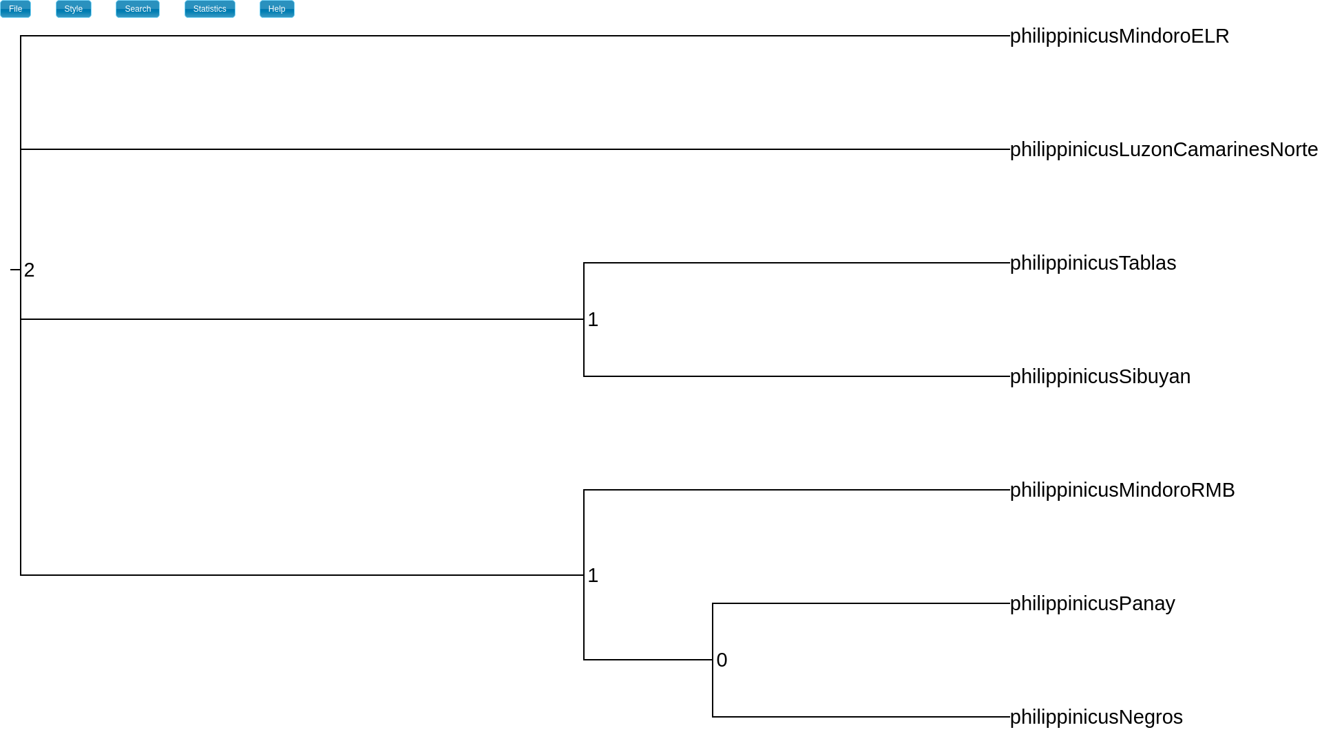
The height_index attribute will show you which nodes share the same divergence times.
If you change the internal node labels to
index_freq
(“Style” -> “Internal node text” -> “index_freq”),
this will display the approximate posterior probabilities for each divergence
event (height).
For example, on my MAP tree, the posterior probability that the two clades with
index “1” share the same divergence time is 0.497.
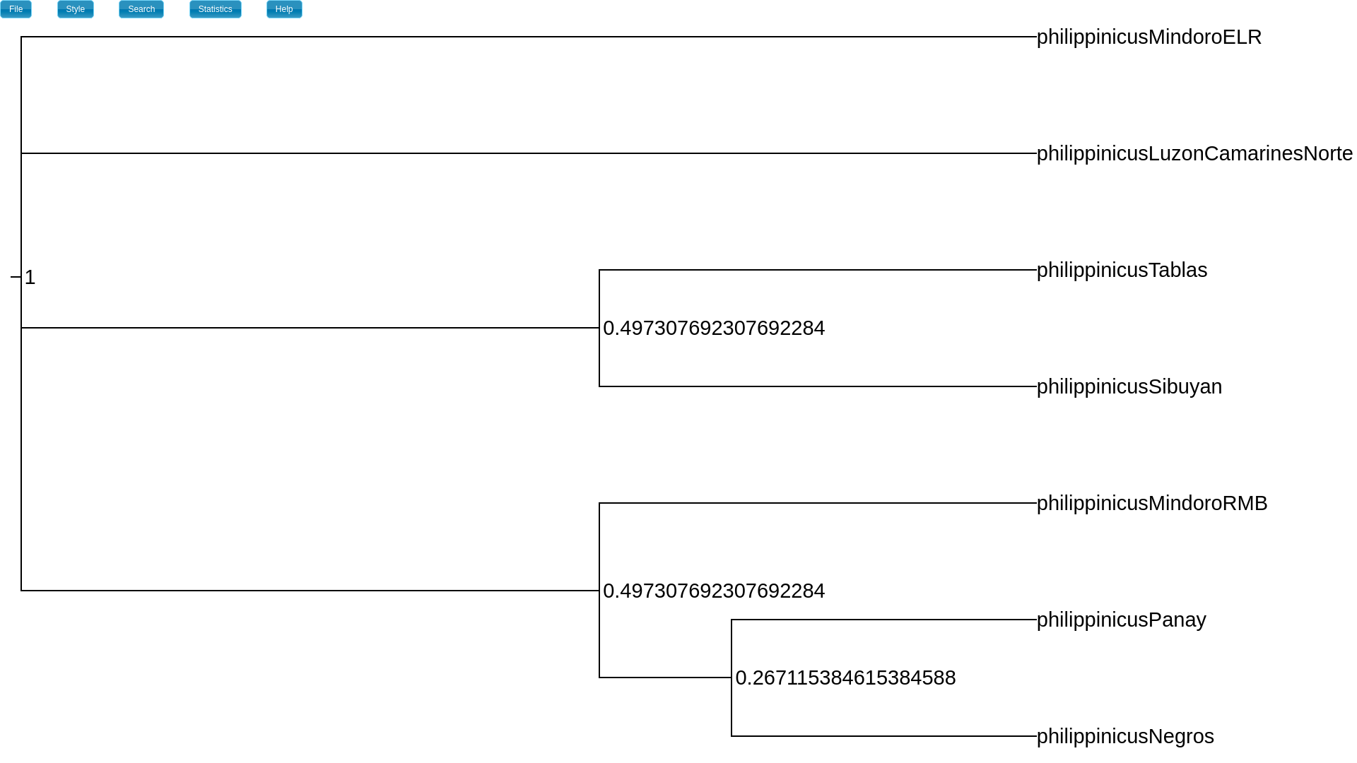
The index_freq attribute is the posterior probability of each
divergence event (height).
If you want to see the Bayesian support values that are typically shown
on trees, change the internal node labels to split_freq.
This will show the approximate posterior probabilities of all the splits
(clades) across the tree.
This is the “normal” support value shown on a tree that summarize the posterior
sample of a Bayesian phylogenetic analysis.
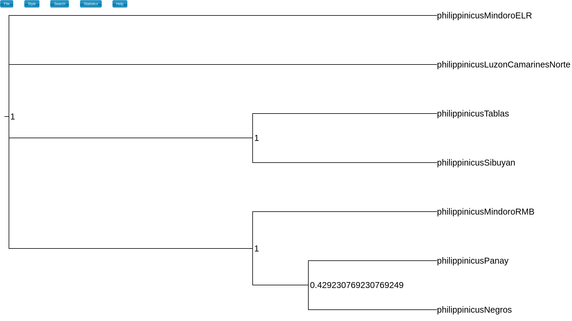
The split_freq attribute is the posterior probability of each split (clade).
However, split (clade) posterior probabilities are not very good at summarizing the support for polytomies (multifurcations) in the tree. To better understand why, please refer to the section above that compares splits versus nodes.
If we want to summarize the support for polytomies, we should look
at the node_freq attribute
(“Style” -> “Internal node text” -> “node_freq”).
This displays the approximate posterior probability of each internal node in
the MAP tree (we define a node by the splits that descend from it).
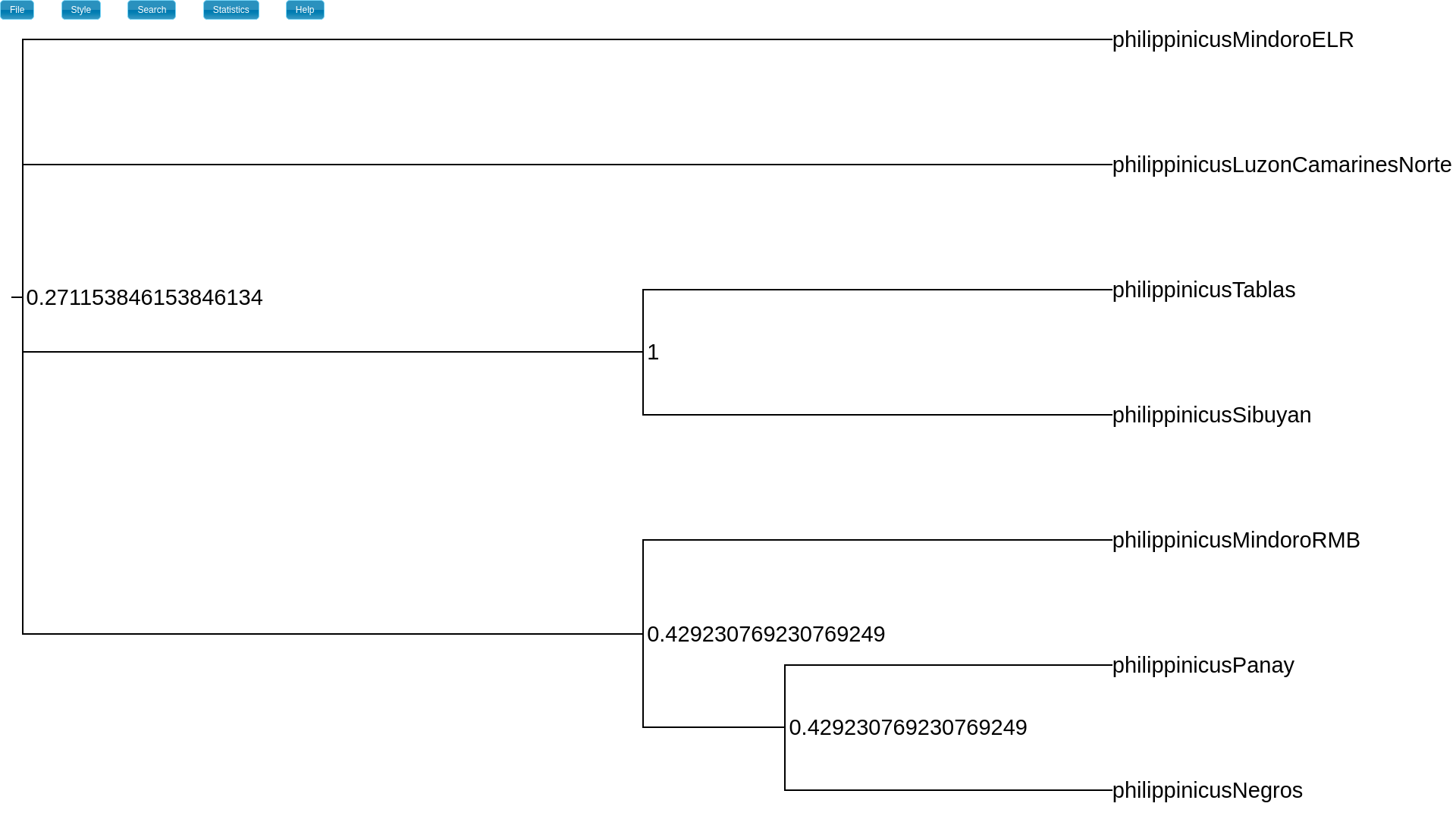
The node_freq attribute is the posterior probability of each node (a
split with a particular set of descendant splits).
In addition to the node attributes above, there are also summaries of the:
Divergence time (height) summarized by divergence event (
index_height_*); i.e., only sampled trees with that particular divergence event (defined by the clades mapped to it) are used to summarize the age of the event.Divergence time (height) summarized by clade/split height (
split_height_*); I.e., all sampled trees that contain the given split are used to summarize the age.Branch length summarized by split (
length_*).Effective population size (
pop_size_*). For this tutorial, this summary is the same for every branch on the MAP tree, because we specifiedequal_population_sizes: truein the phycoeval config file.
The divergence times that are used to “draw” the MAP tree
are the means calculated over divergence events.
By default, the index_height_mean is used, but if the
--median-heights option is specified when running sumphycoeval,
then index_height_median will be used.
Wrap up
After working through this exercise, we hope that we helped you understand
How to prepare data and a configuration file for running phycoeval
How to interpret the output of a phycoeval analysis
The model and computation underlying phycoeval