Sampling the model priors

Important

The most important part of the project is the contents of the ecoevolity configuration files in the ecoevolity-configs directory. These files specify the models we will be using to simulate and analyze genomic datasets.

Read the Background and The ecoevolity configs sections to become familiar with these models.

As described in the Background and The ecoevolity configs sections, we will be analyzing simulated data under three different priors on divergence models:

1. Dirichlet-process (DP) prior

2. Pitman-Yor process (PYP) prior

3. Uniform distribution with a split-weight parameter (SW)

The settings for these models are contained in three ecoevolity configuration files in the ecoevolity-configs directory of the project. These are, respectively:

1. pairs-10-dpp-conc-2_0-2_71-time-1_0-0_05.yml

2. pairs-10-pyp-conc-2_0-1_79-disc-1_0-4_0-time-1_0-0_05.yml

3. pairs-10-unif-sw-0_55-7_32-time-1_0-0_05.yml

Before we do anything else, we should validate that these modes are what we think we are. To do this, we will analyze them with ecoevolity, but tell the program to ignore the data. What should we get if we perform a Bayesian analysis while ignoring the data (i.e., the likelihood is always 1)? The prior!

The config files define the model prior we wish to use. By analyzing it while ignoring the data, the distribution that ecoevolity samples from should be the very one we specified in the configs. Hence, this is a nice sanity check to make sure everything is working as we expect.

Run the analyses

Before anything else, navigate to the project directory (if you are not already there):

cd /path/to/your/copy/of/ecoevolity-model-prior

If you are working on AU’s Hopper cluster, this will be:

cd /scratch/YOUR-AU-USERNAME/ecoevolity-model-prior

Now, lets cd into the project’s scripts directory:

cd scripts

Next, we need to run the prior_sampling_tests.sh script. If you are working on Auburn University’s Hopper cluster, submit this script to the cluster’s queue by entering:

../bin/psub prior_sampling_tests.sh 2

Note

If you are not on the Hopper cluster, you can simply run this directly:

bash prior_sampling_tests.sh 2

Note

If you are on the Hopper cluster, you can monitor the progress of the job by using the qstat command:

qstat

When the script is in queue, but hasn’t started running yet, the output will look like:

Job ID                    Name             User            Time Use S Queue
------------------------- ---------------- --------------- -------- - -----
1941144.hopper-mgt         ...ling_tests.sh jro0014                0 Q general

The second to last column “S” stands for State of the job, and “Q” means it is waiting in queue. When the script starts running, the output of qstat will look like:

Job ID                    Name             User            Time Use S Queue
------------------------- ---------------- --------------- -------- - -----
1941144.hopper-mgt         ...ling_tests.sh jro0014         00:00:40 R general

and the “R” state stands for Running. When the job finishes, the output will look like:

Job ID                    Name             User            Time Use S Queue
------------------------- ---------------- --------------- -------- - -----
1941144.hopper-mgt         ...ling_tests.sh jro0014         00:03:20 C general

where “C” stands for Complete. However, after showing this state for a few minutes, the job will disappear from the output of qstat.

In case you’re curious the “2” argument tells the script how many extra zeros to add to the MCMC chain length specified in the config files. The chain_length in the config files is 75,000 generations. So, the “2” will extend this to 7,500,000. Because, sampling from the prior is fast, we might as well collect a large sample.

What this script will do, is for each of the three model configs listed above, it will:

1. Use simcoevolity to simulate one dataset from that config.

2. Use ecoevolity to analyze that simulated dataset while ignoring the data.

3. Run sumcoevolity to summarize the results.

4. Run pyco-sumevents to plot the results.

5. Run the custom plotting script scripts/plot_prior_samples.py to do some additional plotting of the results.

Why run simcoevolity? I.e., why not just run ecoevolity straightaway? Well the extra step helps to validate that the whole workflow of simulating data and then analyzing them is working as we expect it should. Since we will be doing this thousands of times for this project, it’s a nice extra step for our sanity check.

Checkout the results

Once the prior_sampling_tests.sh script finishes, you should find all of the output for each config file (model) in a prior-sampling-tests directory (assuming you are still in the scripts directory:

ls ../prior-sampling-tests

should reveal:

pairs-10-dpp-conc-2_0-2_71-time-1_0-0_05
pairs-10-pyp-conc-2_0-1_79-disc-1_0-4_0-time-1_0-0_05
pairs-10-unif-sw-0_55-7_32-time-1_0-0_05

Inside of these you will find the dataset simulated by simcoevolity (10 data files; 1 for each pair of populations), the output of ecoevolity (the .log files) and a bunch of plots (.pdf files).

Let’s take a look at the plots from each model and make sure everything looks as we expect.

DPP results

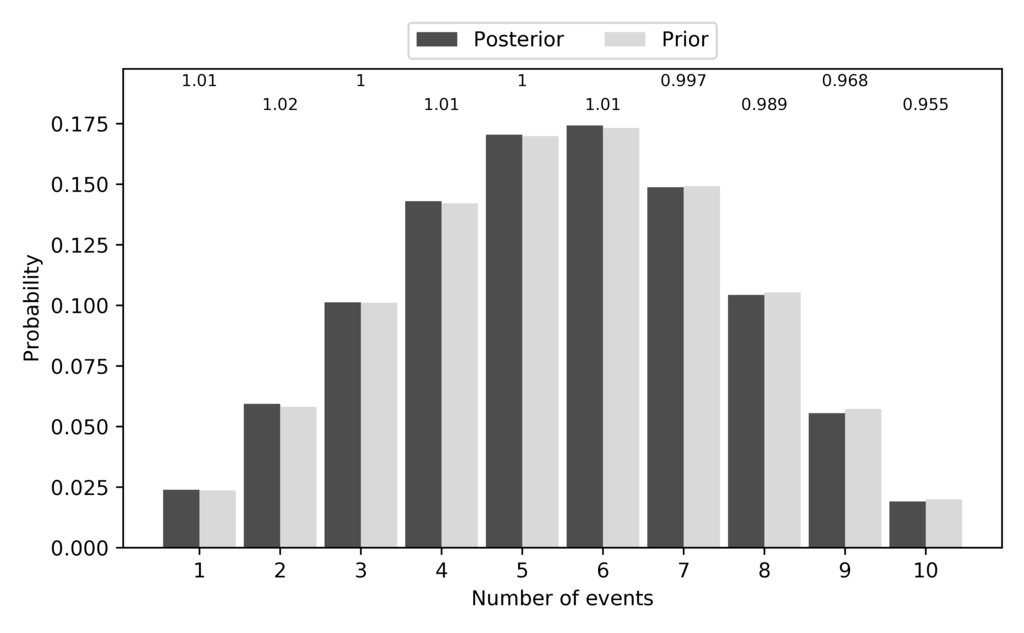
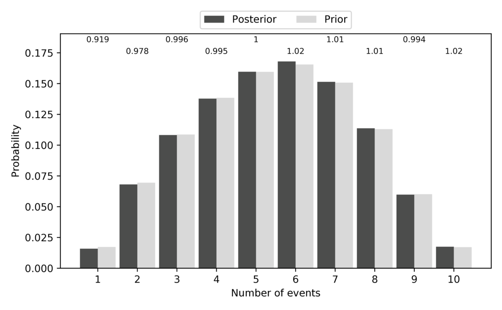
First, let’s look at the plots of the results for the DP model in the ../prior-sampling-tests/pairs-10-dpp-conc-2_0-2_71-time-1_0-0_05 directory. The pycoevolity-nevents.pdf file shows us the how often each number of divergence events was sampled during the ecoevolity analysis. The frequency of samples (dark grey bars) should closely match the expected prior probability of each possible number of events under the model (light grey bars). Note, the dark bars are labeled as “Posterior” in the plot. That’s because when you ignore the data, the posterior should be the prior. So, we want the prior (expected) and posterior (sampled) probabilities of each possible number of events to closely match. Indeed, they do:

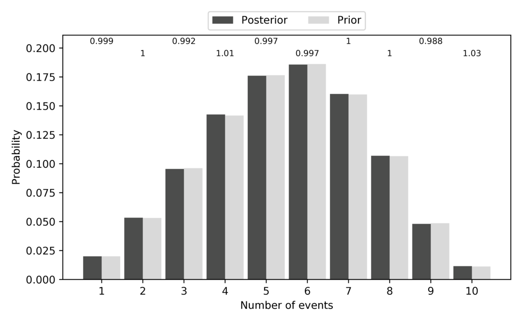
The expected and sampled prior probabilities of the number of divergence events for the DP model.

The prior-concentration.pdf plot shows the expected gamma prior distribution for the concentration parameter (orange line) against a histogram of the values sampled for the concentration parameter during the ecoevolity analysis. It looks like a nice fit:

The expected (orange line) and sampled (histogram) prior distribution on the concentration parameter of the DP model.

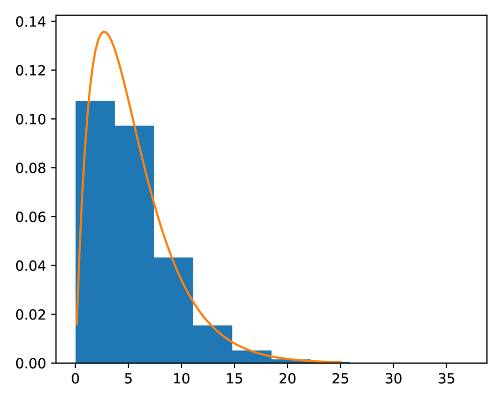
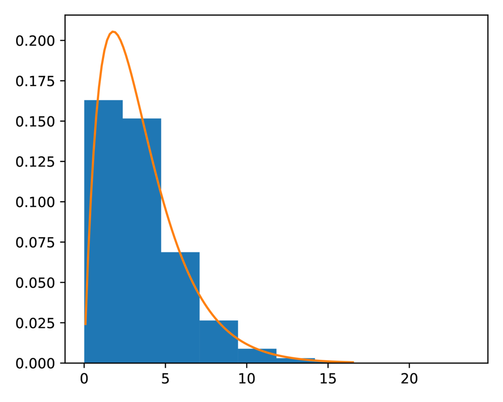
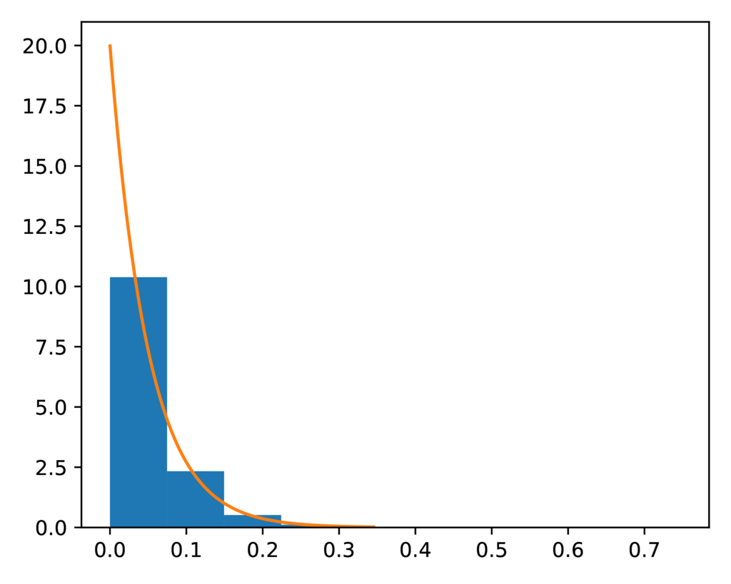
The prior-event_time.pdf plot shows the expected exponential prior distribution on divergence times (orange line) against a histogram of the divergence times sampled during the ecoevolity analysis. It looks like another nice fit:

The expected (orange line) and sampled (histogram) prior distribution on divergence times for the DP model.

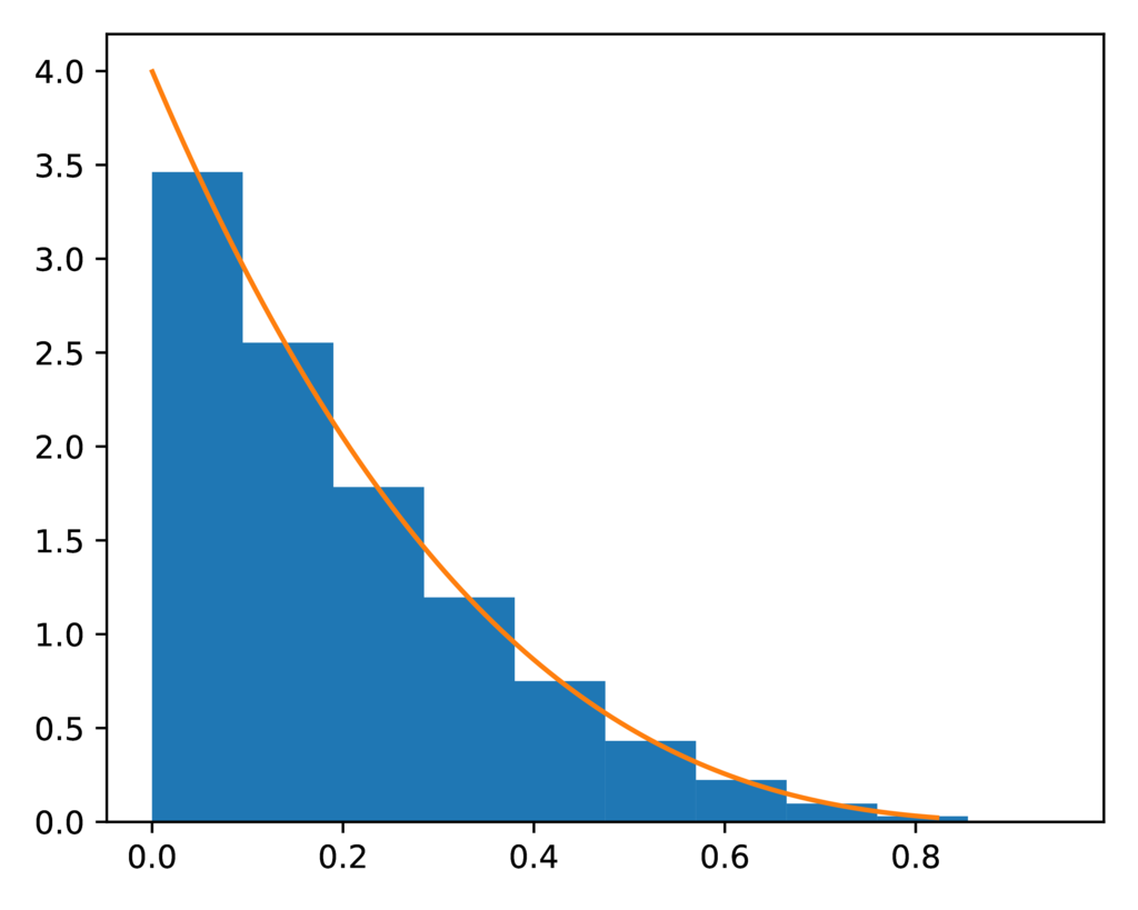
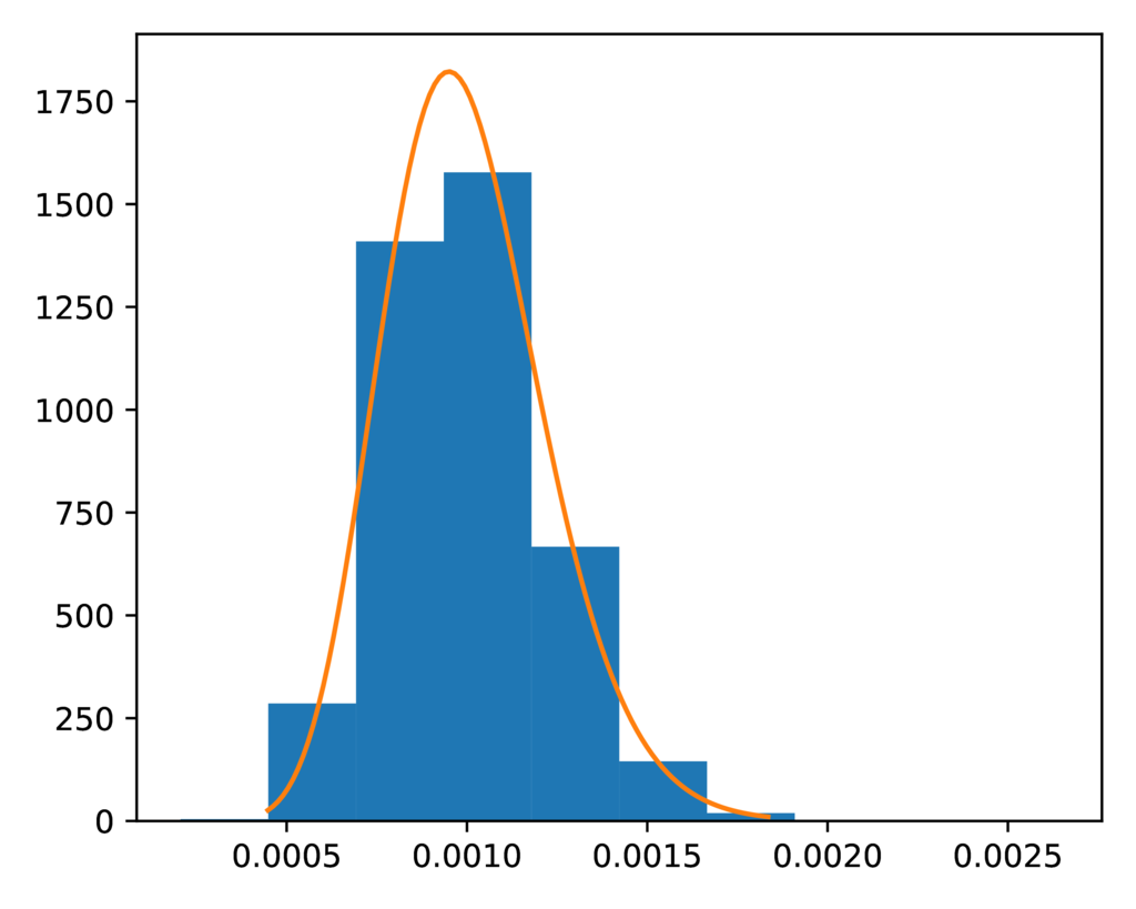
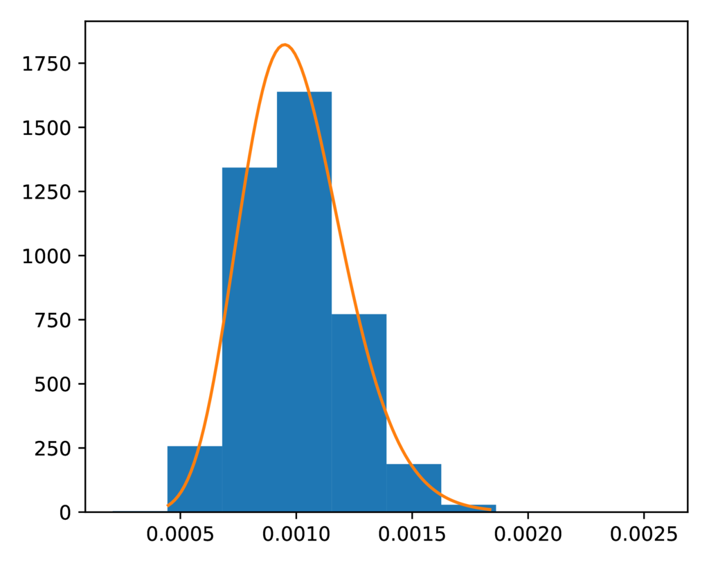
The prior-leaf_population_size.pdf plot shows the expected gamma prior distribution on the effective size of the descendant populations (orange line) against a histogram of the descendant population sizes sampled during the ecoevolity analysis. Bingo:

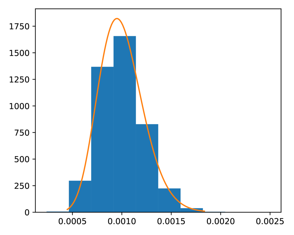
The expected (orange line) and sampled (histogram) prior distribution on the effective size of the descendant populations for the DP model.

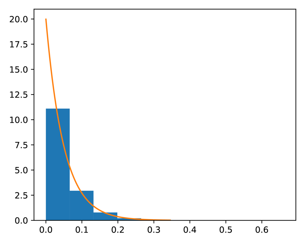
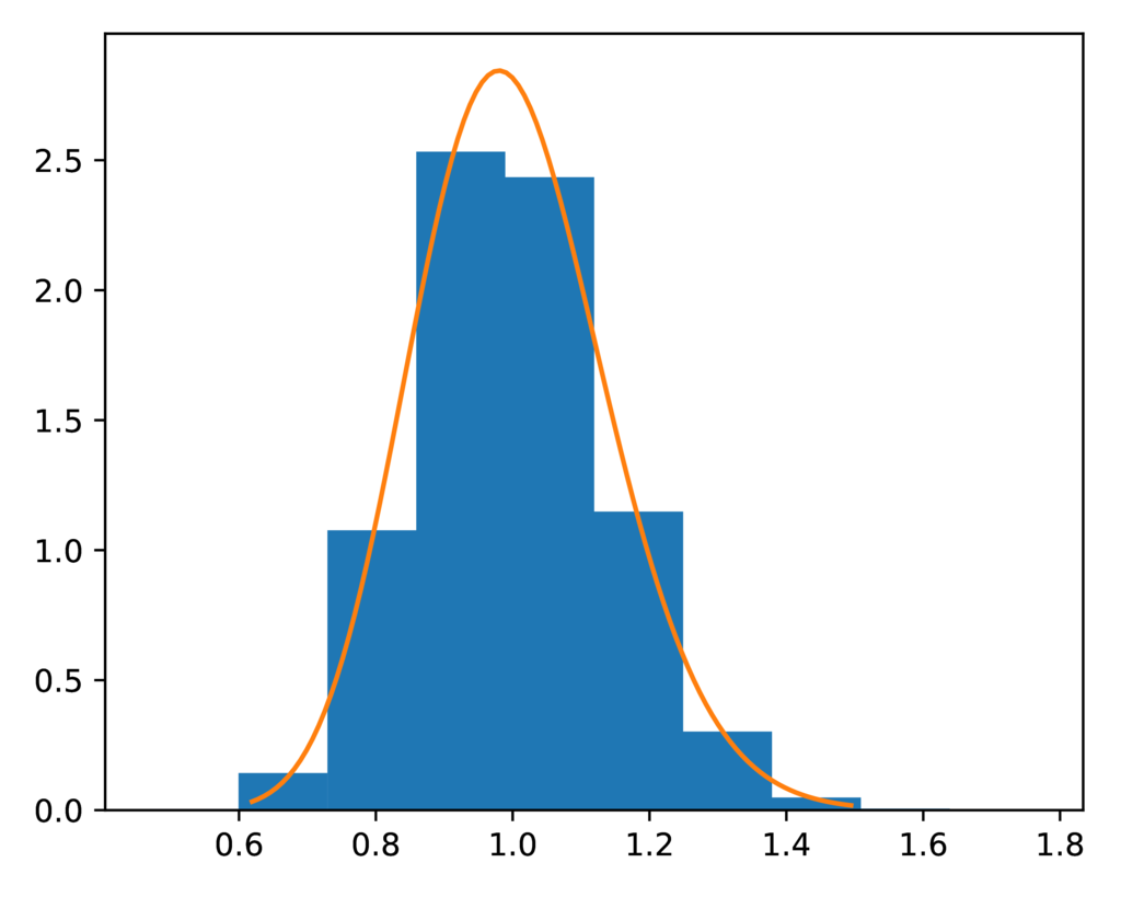
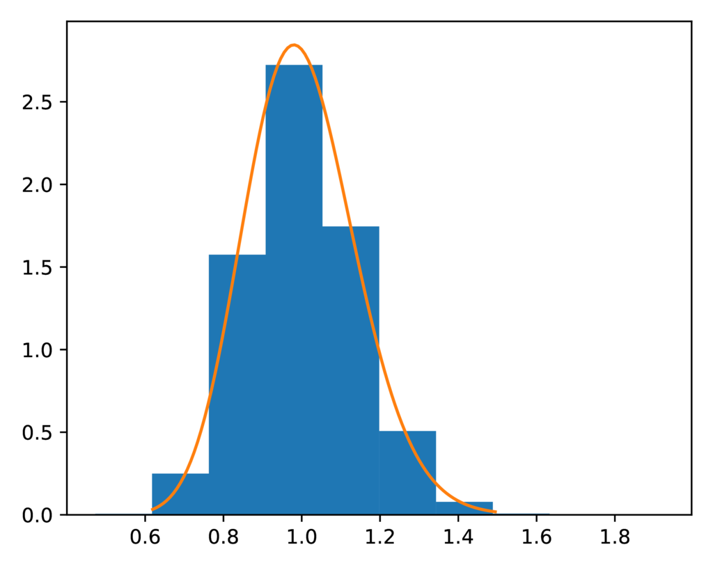
The prior-root_relative_population_size.pdf plot shows the expected gamma prior distribution on the relative effective size of the ancestral population (orange line) against a histogram of the relative ancestral population sizes sampled during the ecoevolity analysis. Spot on:

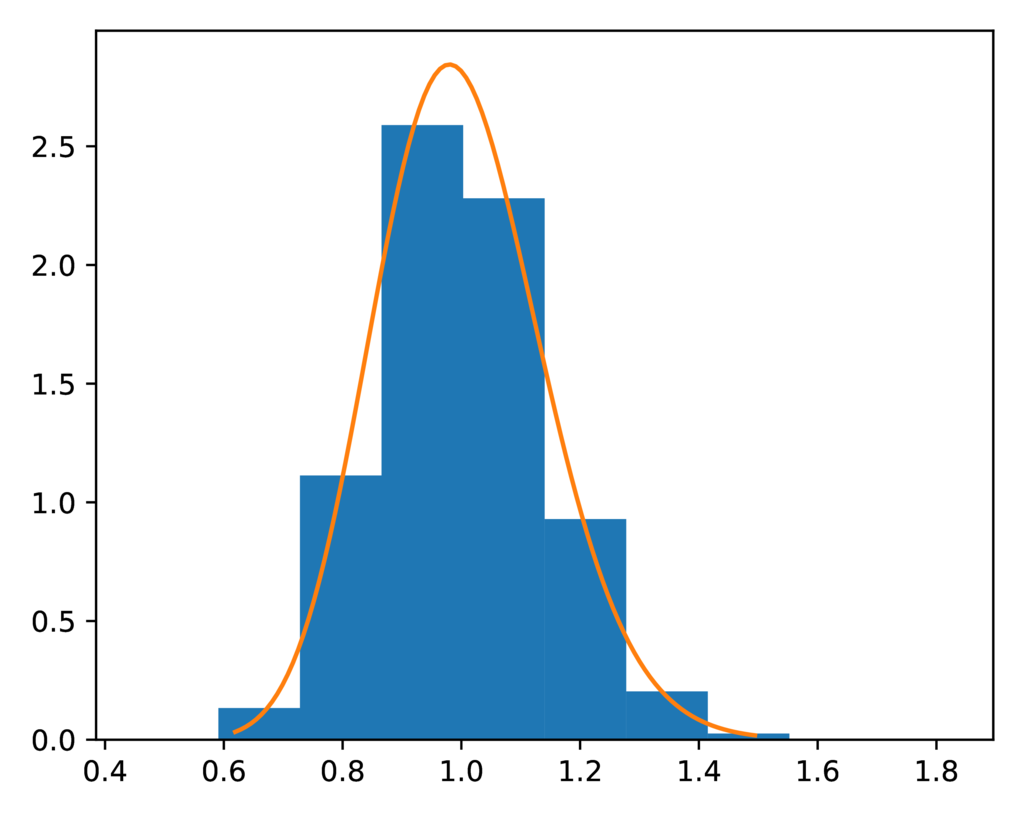
The expected (orange line) and sampled (histogram) prior distribution on the relative effective size of the ancestral population for the DP model.

PYP results

Next, let’s look at the plots of the results for the PYP model in the ../prior-sampling-tests/pairs-10-pyp-conc-2_0-1_79-disc-1_0-4_0-time-1_0-0_05 directory. Just like for the DP model, the pycoevolity-nevents.pdf file shows us the prior (expected) and posterior (sampled) probabilities of each possible number of divergence events. Again, they match nicely:

The expected and sampled prior probabilities of the number of divergence events for the PYP model.

As with the DP model, the prior-concentration.pdf plot shows us that the expected (orange line) and sampled (blue histogram) distribution for the concentration parameter are a close fit:

The expected (orange line) and sampled (histogram) prior distribution on the concentration parameter of the PYP model.

The prior-discount.pdf plot shows the expected beta prior on the discount parameter of the PYP model (orange line) to a histogram of the sampled values for the discount parameter. Another nice fit:

The expected (orange line) and sampled (histogram) prior distribution on the discount parameter of the PYP model.

The prior-event_time.pdf plot confirms the distribution of sampled divergence times closely matches the expected exponential prior distribution on divergence times (orange line):

The expected (orange line) and sampled (histogram) prior distribution on divergence times for the PYP model.

The prior-leaf_population_size.pdf plot confirms the distribution of sampled descendant population sizes closely matches the expected gamma prior distribution:

The expected (orange line) and sampled (histogram) prior distribution on the effective size of the descendant populations for the PYP model.

The prior-root_relative_population_size.pdf plot confirms the distribution of relative sizes of the ancestral populations collected during the ecoevolity analysis closely matches the expected gamma prior distribution:

The expected (orange line) and sampled (histogram) prior distribution on the relative effective size of the ancestral population for the PYP model.

SW results

Lastly, let’s look at the plots of the results for the SW model in the ../prior-sampling-tests/pairs-10-unif-sw-0_55-7_32-time-1_0-0_05 directory.

Just like for the other models, the pycoevolity-nevents.pdf plot confirms that the prior (expected) and posterior (sampled) probabilities of each possible number of divergence events closely match:

The expected and sampled prior probabilities of the number of divergence events for the SW model.

It’s difficult to tell if the distribution of the split-weight parameter approximated by the ecoevolity analysis is a good match to the expected gamma prior distribution:

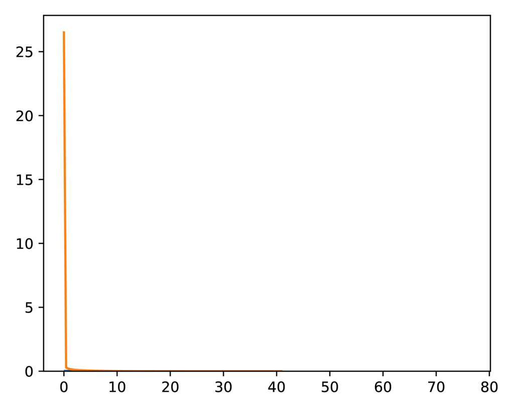
The expected (orange line) and sampled (histogram) prior distribution on the split-weight parameter of the SW model.

This is because it is difficult to approximate a gamma distribution with a shape of 0.55 with a histogram. However, comparing the moments of the distributions confirm a close match. The expected mean of the gamma prior is 4.026, and the mean of the sample collected by ecoevolity is 4.043 The expected variance is 29.47, and the sample variance is 29.50.

The prior-event_time.pdf plot confirms the distribution of sampled divergence times closely matches the expected exponential prior (orange line):

The expected (orange line) and sampled (histogram) prior distribution on divergence times for the SW model.

The prior-leaf_population_size.pdf plot confirms the distribution of sampled descendant population sizes closely matches the expected gamma prior:

The expected (orange line) and sampled (histogram) prior distribution on the effective size of the descendant populations for the SW model.

The prior-root_relative_population_size.pdf plot confirms the sampled distribution of relative ancestral population sizes closely matches the expected gamma prior:

The expected (orange line) and sampled (histogram) prior distribution on the relative effective size of the ancestral population for the SW model.

Summary

These results show that from the output of simcoevolity, ecoevolity will sample from the expected prior distribution described in the config files. This confirms that we don’t have any embarrassing typos in the config files, and that the MCMC algorithms of ecoeovlity are working. These tests do not confirm that simcoevolity will randomly sample datasets from the distributions described in the configs (we only simulated one dataset from each). However, once we simulate lots of datasets from each model, we can check that the samples of parameters from which the datasets were simulated from match the distributions of the models. Also, such checks already exist in the test suite of the ecoevolity software package.

Cleanup

Given how quickly we can generate these results, and the fact that we should regenerate them any time we change/add models to the project, there is no need to add these results to the repository or keep them around. So, once you are done checking out the results, go ahead and remove all of the output:

rm -r ../prior-sampling-tests