Background
The main goal of this project is to explore new ways of modeling shared (temporally clustered) evolutionary events across taxa, and assess the relative performance of these models for inferring such events from comparative genomic data. We have implemented these models in the software package ecoevolity, and so this will be the primary software we use for this project.
The background information below will assume some knowledge of the types of comparative phylogeographic models implemented in ecoevolity. The ecoevolity documentation provides a brief and gentle introduction to such models here. For more details, please refer to [4][6][5].
Ecoevolity models two types of “evolutionary events”: population divergences and changes in effective population size (or “demographic change” for short). Below, and throughout this documentation, we will focus on divergences. Nonetheless, all of comparative models we cover apply to demographic changes (or a mix of divergences and demographic changes) as well.
Let’s use an example to gain some familiarity with the type of inference we will be exploring. Let’s assume we are studying three species (or three pairs of sister species) of lizards that are co-distributed across two islands, and we want to test the hypothesis that these three pairs of populations (or species) diverged when these islands were fragmented by rising sea levels 130,000 years ago. This hypothesis predicts that all three pairs of populations diverged at the same time:
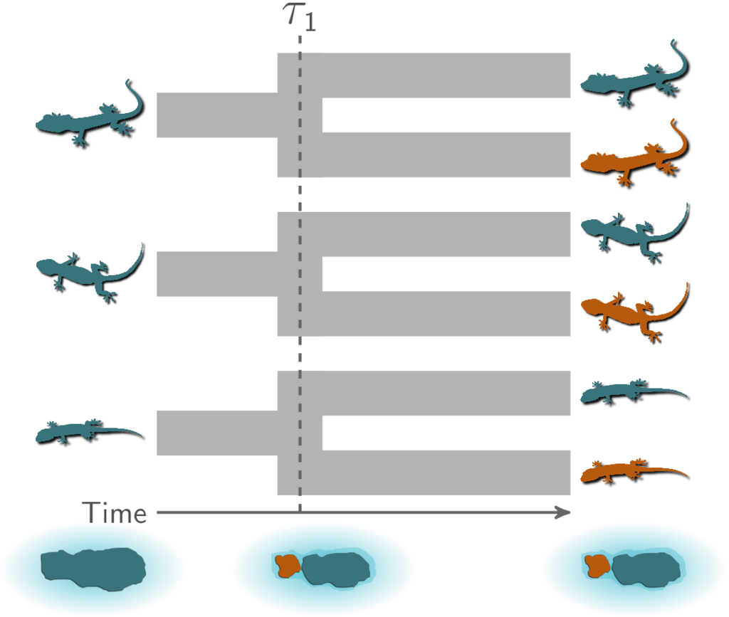
All three pairs of lizard species co-diverged when the island was fragmented.
If we want to evaluate the probability of such a model of co-divergence, we also need to consider other possible explanations (i.e., models). For example, perhaps all of these populations were founded by over-water dispersal events, in which case there is not obvious prediction that these events would be temporally clustered. Rather we might expect the dispersal events to have occurred at different times for each species. Or maybe two pairs of populations co-diverged due to sea-level rise, but the third at a different time via dispersal.
So, there could have been 1, 2, or 3 divergence events in the history of our lizard populations. If there was 1, all three pairs of populations diverged at the same time. If there were 3, they all diverged at unique (independent) times. If there were 2, two diverged at the same time and other diverged independently. For this last scenario, the pair of populations that diverged independently could have been any of our three pairs. So with three pairs, there are a total of 5 possible models explaining their history of divergence times.
If we want to take a Bayesian approach to comparing these 5 models, we need away to assign prior probabilities to all 5 models; that is, how probable we think each model is before we look at comparative genomic data from these populations. This seems quit trivial with only 5 possible models. However, the number of possible models increases quickly as we add more taxa to our study. So, we would like a way of assigning prior probabilities to all possible models of divergence that is fast and flexible. Flexibility is desirable, because it would allow us to incorporate prior information (or lack thereof), or integrate over uncertainty in such prior assumptions.
Priors on divergence models
Dirichlet-process prior
The original implementation of ecoevolity treated the divergence model (number of
divergence events, and the assignment of the taxa to the events) as a random
variable under a Dirichlet process (DP) [2][1].
At its core, the Dirichlet process is simple; we assign
elements (pairs of populations)
to
categories (divergence events)
one at a time following a simple rule.
When assigning the  pair, we assign it to its own event (i.e., a
new divergence event with a unique time) with probability
pair, we assign it to its own event (i.e., a
new divergence event with a unique time) with probability
(1)
or we assign it to an existing event  with probability
(2)
where  is the number of pairs already assigned to
event .
is the number of pairs already assigned to
event .
For example, let’s apply this rule to our three pairs of lizard populations.
First, we have to assign our first pair (“A”) to a
divergence event with probability 1.0;
let’s call this the “blue” divergence event.
Next we assign the second pair (“B”) to either a new (“red”) divergence
event with probability  or to the same “blue”
divergence event as the first pair with probability
or to the same “blue”
divergence event as the first pair with probability  .
For this example, let’s say it gets assigned to the “blue” event.
Lastly, we assign the third pair (“C”) to either a new (“red”) divergence
event with probability
.
For this example, let’s say it gets assigned to the “blue” event.
Lastly, we assign the third pair (“C”) to either a new (“red”) divergence
event with probability  or to the same “blue”
divergence event as the first two pairs with probability
or to the same “blue”
divergence event as the first two pairs with probability  .
.
The animation below illustrates how the these simple rules determine the prior probability of all five possible models of divergence. Notice toward the end of the animation, as the concentration parameter increases we place more probability on the divergence models with more independent divergence events (less shared divergences).
An example of the Dirichlet process.
Click here for a larger, interactive demonstration of the DP.
The DP gives us a way to quickly calculate the prior probability of any divergence model given a value of the concentration parameter. You might notice that the order of the elements does not affect the probability. This property of the DP (exchangeability) allows us to use Gibbs sampling [3] to sample across divergence models. Also, the concentration parameter makes the DP flexible. We can adjust the concentration parameter to fit our prior expectations regarding the probabilities of the divergence models, and we can put a distribution on the concentration parameter and integrate over uncertainty about the prior probabilities of the divergence models.
Pitman-Yor process prior
One of the newly implemented ways of modeling shared divergences is
the Pitman-Yor process (PYP) [7].
The PYP is a generalization of the Dirichlet process.
It adds an additional parameter called the “discount” parameter, which
we will denote as  .
When
.
When  the PYP is equivalent to the DP.
The discount parameter give the PYP flexibility over the tail behavior of the
process (the DP has exponential tails).
the PYP is equivalent to the DP.
The discount parameter give the PYP flexibility over the tail behavior of the
process (the DP has exponential tails).
The rule governing the PYP is very similar to the DP.
When assigning the pair, we assign it to its own event (i.e., a
new divergence event with a unique time) with probability
(3)
where  is the number of events that currently exist (i.e., that
already have a pair assigned to it).
Or, we assign it to an existing event with probability
is the number of events that currently exist (i.e., that
already have a pair assigned to it).
Or, we assign it to an existing event with probability
(4)
where is the number of pairs already assigned to
event .
The animation below illustrates how the these rules of the PYP determine the prior probability of all five possible models of divergence. Notice toward the end of the animation, as the discount parameter increases we place more probability on the divergence models with more independent divergence events (less shared divergences). Again, when the discount parameter is zero, the PYP is equivalent to the DP.
An example of the Pitman-Yor process.
Click here for a larger, interactive demonstration of the PYP.
With an extra parameter, the PYP has greater flexibility than the DP. We can adjust both the concentration and discount parameters to fit our prior expectations. Also, we can put distributions on both of these parameters and integrate over uncertainty about the prior probabilities of the divergence models. The PYP preserves the mathematical conveniences of the DP. We can quickly calculate the probability of any model, and the exchangeability property still allows us to use Gibbs sampling to sample across possible divergence models.
Uniform prior
We have also implemented a uniform prior over divergence models, where we
assume a priori that every possible divergence model (every way of grouping
the divergence times of the population pairs) is equally probable.
Furthermore, we added a “split weight” parameter, which we denote as  ,
to provide some flexibility to this prior on divergence models.
,
to provide some flexibility to this prior on divergence models.
We can think of the split weight () in simple terms.
For a given model with divergence events (i.e., divergence time
categories), the relative probability of each model with
 events is ,
and the relative probability of each model with
events is ,
and the relative probability of each model with
 events is
  .
More generally, the relative probability of each model with
.
More generally, the relative probability of each model with
 events is
  ,
and the relative probability of each model with
,
and the relative probability of each model with
 events is
  .
.
To get a feel for this “uniform” prior, in the following tables we will look at an example for 4 pairs of populations, with 3 different values for the split weight. First, some notation that is used in the tables:

The number of population pairs we are comparing.
The number of divergence events (i.e., divergence time categories).

The number of models that have
categories (the Stirling number of
the second kind).
The relative probability of each model with
events (we scale this
relative probability to help make the tables readable).
The relative probability of the entire class of divergence models with
events.
The probability of each divergence model with
events.
Split weight  :
:
|
|
|
|
|
1 |
1 |
1 |
1 |
|
2 |
7 |
1 |
7 |
|
3 |
6 |
1 |
6 |
|
4 |
1 |
1 |
1 |
|


Split weight  :
:
|
|
|
|
|
1 |
1 |
1 |
1 |
|
2 |
7 |
2 |
14 |
|
3 |
6 |
4 |
24 |
|
4 |
1 |
8 |
8 |
|


Split weight  :
:
|
|
|
|
|
1 |
1 |
8 |
8 |
|
2 |
7 |
4 |
28 |
|
3 |
6 |
2 |
12 |
|
4 |
1 |
1 |
1 |
|


The Goal
Our primary goal with this project is to compare the performance of the Dirichlet-process, Pitman-Yor, and uniform priors when inferring shared divergences from comparative genomic data. To do this, we will simulate datasets under each of these three models (as well as models that violate all three of them) and then analyze each simulated dataset under each of these three models to compare the accuracy, precision, and robustness of the estimated timing and sharing of divergences.